This project aims to classify food into different types based on nutrient composition.
Three Machine Learning techniques will be used for this multi-class classification problem:
- Random Forest
- Support Vector Machine (SVM)
- Multilayer Perceptron (MLP)
Hyperparameters will be tuned, and other ways will be explored to improve them. Also, I will compare the classifier using PCA and without PCA to determine which classifier performs better.
10-fold cross-validation will be used on the training set to evaluate the classifier’s performance. Also, the accuracy of the test set will be used to evaluate how well the classifier performs, especially on unseen data and how well the classifier is generalised to new data.
Exploratory Data Analysis and Data Pre-processing:
The dataset has 289 unique classifications, making it difficult to include them all. Thus, I selected three classes from the dataset. Two approaches were trialled to determine which food classes would be the best for the new dataset.
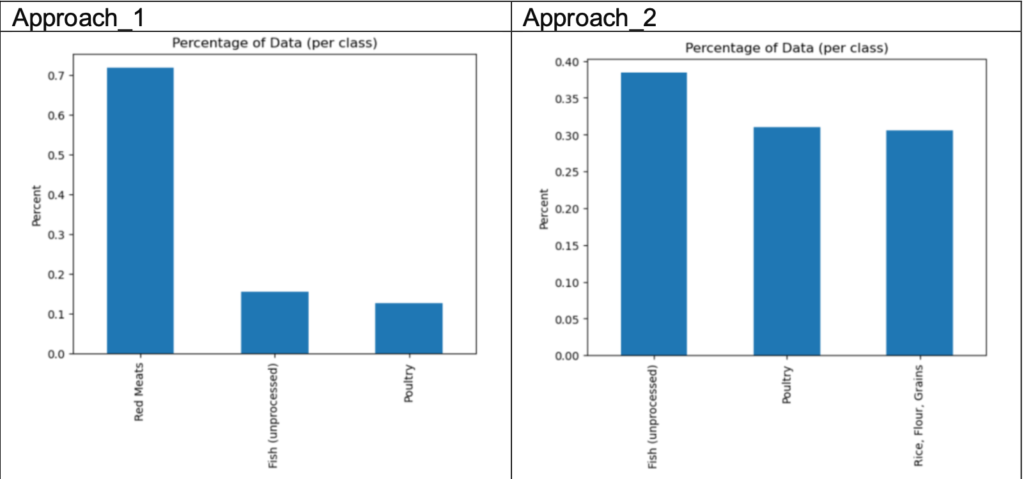
Based on the plot, if we choose the following classes from approach_1 as the new dataset, it may cause imbalanced data as the red meat class has significantly more samples (approximately 70%) than the other two classes (15% for each class), which can cause the classifiers later to be biased towards the majority class and perform poorly on the minority class. For approach 2, the ratio of each class is approximately 0.4 (Fish) : 0.3 (Poultry) : 0.3 (Rice, Flour, Grains), which is almost equivalent and may avoid imbalanced data. Thus, the second approach was chosen, and there are 190 samples.
We do not consider the remaining classes because most of them have a small number of samples, which may lead to overfitting, poor generalisation, and high variance in model predictions. Thus, the remaining classes were removed.
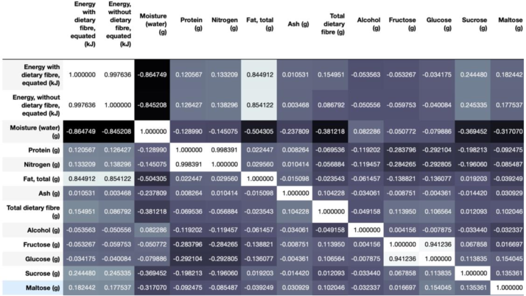
Correlation Matrix (Only part of the features as unable to capture all of them):
There are many features that are highly correlated, such as Protein and Nitrogen, and Glucose and Fructose. These are reasonable because nitrogen’s role in protein synthesis and glucose and fructose has very similar molecular structures, so each pair of highly correlated features are expected to affect each other directly.
Next, remove the features that have all missing values and zeros. Impute the remaining features with mean value if there is a missing value. Encode the target labels via the LabelEncoder from sklearn library with values between 0 and 2, with Fish being 0, Poultry being 1, and “Rice, Flour, Grain” being 2.
Randomly shuffle the dataset and split them into 70% for training and 30% for testing. The train_test_split was completed using a random_state parameter set to 42, so we will get the same split each time.
Perform a standardisation for the features (X_train & X_test). Some features may have values greater than 1000, and some may have values as low as 0.001, so implementing standardisation ensures all features contribute equally to the models and prevents features with larger values from dominating the models later and leading to biased results.
Dimensionality Reduction (PCA):
A dimensionality reduction technique called principal component analysis (PCA) transforms a set of features from a dataset into a fewer number of features called principal components while preserving as much information as possible from the original dataset. It can remove correlated features, improve machine learning algorithm performance and reduce overfitting. The limitation of PCA is that it will cause information loss, and the independent variables are now less interpretable. PCA was implemented using the sklearn library and only on the features.
Random Forest:
Random forest is widely used for classification problems and can handle high-dimensional data with numerous features and datasets with missing values and outliers.The benefit of random forest is that it reduces the risk of overfitting, which happens when the classifier performs well on the training data but poorly on new, unseen data. Random forest achieves this by constructing multiple decision trees on subsets of the data and then combining the results, thereby lowering the impact of individual trees that may have to overfit the data.
The two main parameters that will be tuned are n_estimators (number of trees) and max_depth (maximum depth allowed for each tree). Tuning the n_estimators and max_depth hyperparameters of Random Forest can maximise classifier performance, prevent overfitting, and strike the right balance between complexity and generalisation.
Firstly, I ran two classifiers (PCA and without PCA) with the default hyperparameters. Then, I used RandomizedSearchCV for PCA and without PCA to find the best hyperparameters (n_estimators and max_depth) for each classifier. RandomizedSearchCV is a hyperparameter optimisation technique that randomly samples a subset of hyperparameter combinations from a predefined search space to efficiently tune classifiers and find the best-performing configuration.
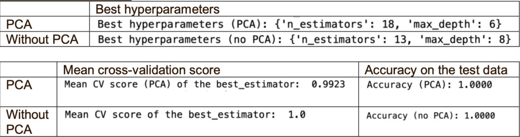
When using the best hyperparameters, PCA performs better than without PCA. One reason could be that the PCA classifier might be overfitting the training data.
Confusion Matrix (without PCA with best hyperparameters):
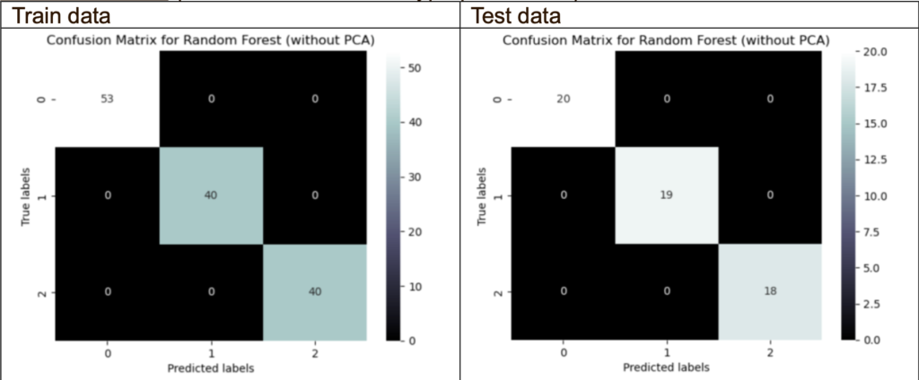
The confusion matrix without PCA shows no misclassifications on the train and test data. This may mean that the classifier’s performance accurately predicts the target variables.
Decision boundaries plot (using 2 principal components only):
The objective for this part is to look at the decision boundary plot; however, I will also include the accuracy and cross-validation scores.
The PCA classifier with 2 principal components performs poorly compared with the one without PCA and the PCA with 24 principal components. Based on the decision boundary plots, both the train and test sets suffer from slight overfitting as did not generalise well to new unseen data. The reason could be that the explained variance for 2 principal components is 24.3%, leading to a loss of information compared with the original features. Thus, limiting the classifier’s ability to learn and generalise accurately.
Importance of each feature:
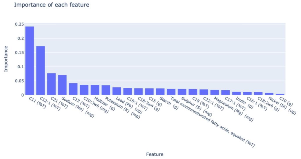
This plot tells us that C11 (%T) was the biggest predictor of the classifier in determining which type of food it could be, followed by C12 (%T). C20 (g) has the least contribution when predicting the type of food.
Support Vector Machine (SVM):
SVM is effective in high-dimensional spaces, making it an excellent option for classification problems involving many features. This is because SVM uses a kernel function to map the input data to a higher-dimensional space where a hyperplane can separate the classes. The benefits of SVM for high-dimensional classification problems include improved performance, higher accuracy, and shorter training times.
The two main parameters that will be tuned are kernels (linear, RBF, polynomial) and C values. The linear kernel is used for linear classification, and RBF and polynomial kernels could fit non-linear relationships. The C value could control the hardness or softness of the margin between the classes. A smaller C value results in a softer margin, and a larger C value enforces a hard margin.
Firstly, I ran two classifiers (PCA and without PCA) with the default hyperparameters. Then, I used GridSearchCV for PCA and without PCA to find the best hyperparameters (kernel and C value) for each classifier. There were 5 options for the C values, which are 0.01, 0.1, 1.0, 10, 100.
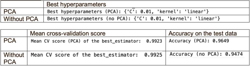
When using the best hyperparameters, PCA performs better than without PCA as it has higher accuracy, although the mean cross-validation score is slightly lower. One reason is that the mean cross-validation scores are much higher than the accuracy is the limited samples (total 190 samples only), which could not generalise well to the unseen data. Another reason could be overfitting the training data when using the best hyperparameters.
Confusion Matrix (PCA with the best hyperparameters):
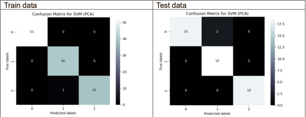
The majority of the data are able to accurately predicts the target variables. However, there is one misclassification in the train data and 2 misclassifications in the test data.
Try different kernels:
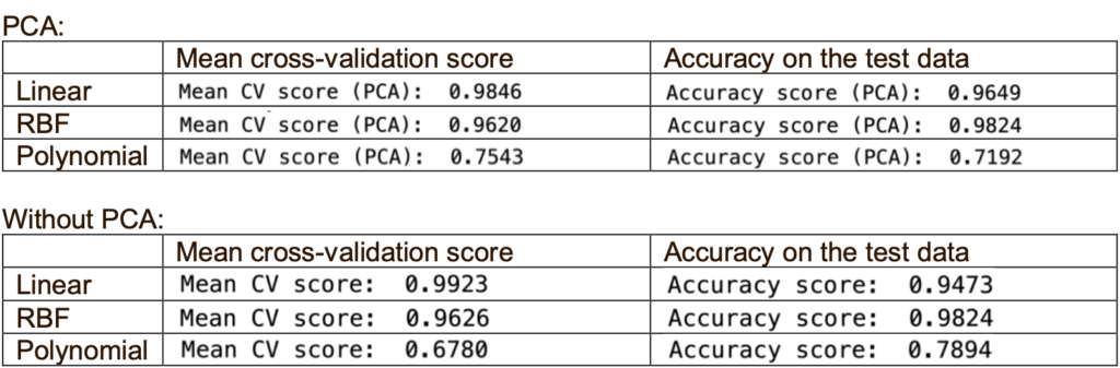
Based on the accuracy, the RBF kernel is the best for PCA and without PCA. Based on the cross-validation score, the linear kernel will be the best. Both linear and RBF kernels performed comparably well except for the polynomial kernel.
Try C value using the different kernels (Using PCA):
The linear kernel’s optimal C value starts at 0.1, showing a preference for larger margins and a lower chance of overfitting. The optimal C value for the RBF kernel starts at 1.0, enabling more intricate decision boundaries. The polynomial kernel shows the best performance with C values starting at 100, allowing greater flexibility in capturing non-linear relationships.
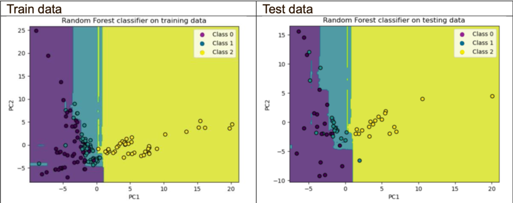
Decision boundaries plot (using 2 principal components only):
The objective for this part is to look at the decision boundary plot; however, I will also include the accuracy and cross-validation scores.
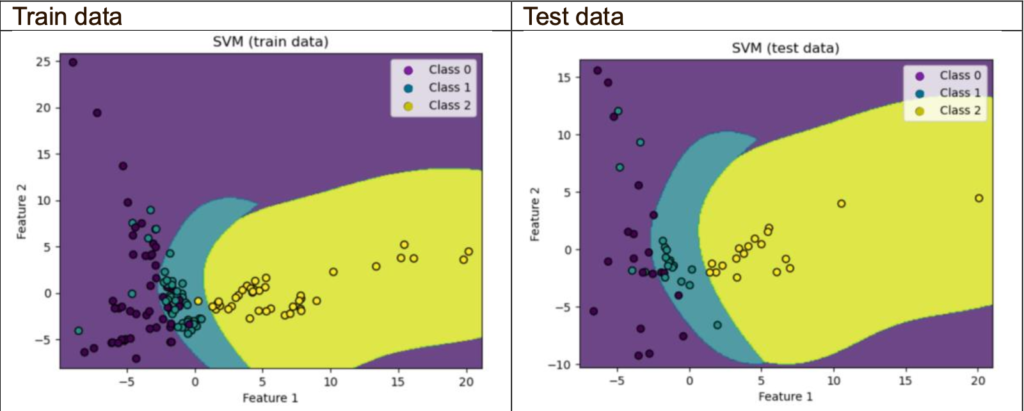

The PCA classifier with 2 principal components performs as well as the one without PCA and the PCA with 24 principal components. There is no overfitting but very slight underfitting. It could be due to the non-linear relationship, which means the PCA uses a linear dimensionality reduction technique, and the SVM of the RBF kernel is suitable for non-linear data when it comes to the non-linear kernel.
Multi-Layer Perception (MLP):
MLP contains a variety of interesting hyperparameters that I was interested in tuning to improve the behaviour of the classifier. Moreover, extending MLPs to deeper architectures with more hidden layers is possible. It could learn hierarchical representations of data, which can help identify complex patterns and obtain higher accuracy.
The three parameters that will be tuned are activation (relu, tanh, logistic), learning rate and hidden layer. This activation function computes how a layer’s input values are presented in the output value. The learning rate controls the weight at the end of each batch.
Firstly, I ran two classifiers (PCA and without PCA) with the default hyperparameters. Then, I used GridSearchCV for PCA and without PCA to find the best hyperparameters (activation, learning rate, hidden layer) for each classifier. There were 4 options for the learning rate, which are 0.0001, 0.001, 0.01, 0.1.
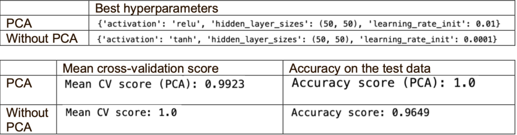
The best activation for PCA is relu, and without PCA is tanh. One reason that tanh activation is the best activation for without PCA is that it may be more appropriate for the nature and scale of the original features.
When using the best hyperparameters, PCA performs better than without PCA as it has higher accuracy, although the mean cross-validation score is slightly low. One reason could be the limited samples, which may cause overfitting as the classifier did not learn generalised patterns but memorised the training data. Without PCA, the mean cross-validation score is slightly higher than the accuracy. This could be due to overfitting the training data using the best hyperparameters.
Confusion Matrix (PCA with the best hyperparameters):
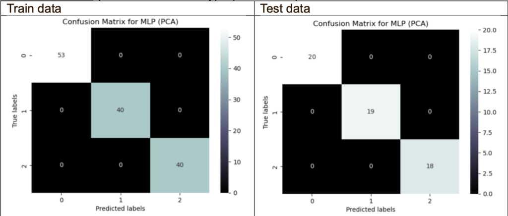
The confusion matrix of PCA shows no misclassifications on the train and test data. This may mean that the classifier’s performance accurately predicts the target variables.
Try different activations (Using PCA):
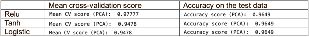
Tanh and Logistic activations have the same accuracy and mean cross-validation scores. It may be because Tanh and Logistic are similar, such that they are sigmoid functions, and both can suffer from vanishing gradients.
Try learning rate using the different activation (Using PCA):
If the learning rate is too low, it will lead to slower convergence as it requires more iterations to converge (find the optimal solution) and may lead to underfitting. If the learning rate is too high, it can lead to overshooting the optimal results and failing to converge.
It seems like the learning rate equal to 0.01 is the optimal learning rate for the three activations. When it comes to a learning rate equal to 0.1, the classifier may have issues converging or settling into a suitable region of the parameter space, leading to suboptimal performance and lower accuracy.
Conclusion:
For this project, I managed to find the best classifiers using different machine-learning techniques and tried tuning different hyperparameters for the classifiers. Random Forest, without the PCA classifier, outperformed the PCA classifier. For SVM and MLP, both the PCA and without PCA classifiers generally performed well.
However, based on the results above, I realised that without PCA classifiers could perform better than PCA classifiers. Hence, PCA may not be suitable and necessary for this dataset.